
Multiple Linear Regression in Power BI
In this post, I will describe how to implement Multiple Linear Regression in Power BI using DAX only.
In the February 2023 release, Power BI introduced a new function called “Linest“, so we will see how to use it to make predictions and interpret its result.
Table of Contents
Linear Regression
Linear regression is a type of statistical analysis used to find the relationship between two variables. It is used to determine how one variable (dependent variable) is related to another variable (independent variable).
The aim of linear regression is to find a straight line that best fits the data points on a scatter plot. Once the regression line is determined, we can use it to estimate the values of the dependent variable based on the values of the independent variable.
A common algorithm used to find the regression line is called “least squares”.
Multiple Linear Regression
Multiple linear regression is an extension of simple linear regression. Instead of analyzing the relationship between two variables, it analyzes the relationship between one dependent variable and multiple independent variables. Instead of finding a line that best fits the data points on a scatter plot, multiple linear regression finds a plane or hyperplane that best fits the data points.
So simply, multiple linear regression allows us to make predictions based on a relationship between one dependent variable and multiple independent variables.
Least Square
While linear regression is a statistical technique that aims to model the relationship between variables, Least squares, on the other hand, is a method used in linear regression to find the line or curve that best fits a set of data points. It works by minimizing the sum of the squared differences between the actual values of the dependent variable and the predicted values based on the regression line or curve.
To see in more detail how this equation works you can refer to a previous post where I described how to calculate the CORRELATION COEFFICIENT IN POWER BI USING DAX, the equation used in this post was the least square so now this post is kind of obsolete since we can directly use the new Linest function instead of writing the whole formula in DAX 🙂
Implement the Multiple Linear Regression in Power BI
Before starting to implement the Multiple Linear Regression in Power BI let’s take a look at the data and describe the scenario.
The Data
To make things easy to follow and easy to implement I wanted to use a simple and small dataset with enough variables and at least one categorical variable.
So in this scenario, we will try to predict monthly sales of the Hyundai Elantra car in the United States. The Elantra Sales dataset is widely used in statistics courses.
Here are the variables included in our dataset:
- ElentraSales: The dependent variable that we will try to predict
- Year: Year of the sales
- Month: Month of the sales
- Unemployment: % of unemployment in the US
- CPI_energy: the monthly consumer price index (CPI) for energy
- CPI_all : the consumer price index (CPI) for all products
- Queries: number of Google searches for “hyundai elantra”
In this dataset, we have the monthly sales of the ELentra car from 2010 to 2013, there are 6 independent variables and 48 rows.

The DAX function
The DAX function is very simple to write, the first parameter to pass is the dependent variable then all the next columns will be the independent variables used for predicting the dependent variable. This function will then generate a calculated table.
Interpret the output
The output of the calculated table is as follows:

The first thing that I don’t like with the output and that I believe could be improved in the future is that the names of the columns are not mapped to the input column names so we need to rename all the columns’ output to make the calculated table easier to interpret and reuse after.
Let’s rename all the columns:

Now let’s explain the output:
Coefficient of Determination
Probably the most important metric for the model is the coefficient of determination or more commonly called the “R2”. It is a number between 0 and 1 that measures how well a statistical model predicts an outcome so the higher the better.
Degree Of Freedom
Degrees of freedom or DF refers to the number of values in a calculation that is free to vary, given certain constraints or limitations.
The formula to find the DF is N (sample size) – P (number of parameters or input variables) thus in our scenario it is 48 rows – 6 variables=42.
DF is important for finding critical cutoff values in inferential statistical tests, as a rule of thumb the higher the DF is the better as it gives more power to reject a false null hypothesis.
FStatistics
In regression, the F-statistics is used to test the significance of the model so generally, if the F-statistics is larger than the F-critical value (according to the desired significance level usually 95%) we can be confident to reject the null hypothesis.
In our scenario, the F-critical value is around 2.335 according to the F-table (df1=6, df2= 41 for alpha 0.05), as our F-stats 8.64 is much larger than the F-crit value we can confidently reject the null hypothesis.
The F-stat can be obtained with the following formula, F-stat=Mean sum of squares regression (MSR) / Mean sum of squares error (MSE)
Regression Sum Of Squares
The RegressionSumOfSquares also called SSR is used to describe how well a regression model represents the modeled data. A higher regression sum of squares indicates that the model does not fit the data well.
The SSR is also used to compute the Mean sum of squares regression (MSR).
Residual Sum Of Squares
The residual sum of squares or also called SSE is a measure of the differences between the actual and predicted values in a regression model. It represents the amount of variation in the dependent variable that cannot be explained by the model. A smaller SSE value suggests that the model is better at explaining the data. The SSE is also used to compute the Mean sum of squares error (MSE).
Intercept
The intercept (often labeled as constant) is the point where the function crosses the y-axis.

In multiple linear regression, the intercept is the mean for the response when all of the explanatory variables (independent variables) take the value of 0.
Slope
The slope coefficients in multiple regression show how the dependent variable changes on average for each one-unit increase in the independent variable while keeping other independent variables constant. For instance, in our example, the slope for the “Year” variable is 9,889, meaning that, on average, for every one-unit increase in the “Year” variable, the dependent variable (sales) is expected to increase by 9,889 units while other variables are constant. Similarly, if the slope coefficient for “Unemployment” is -2,225, this indicates that, on average, for every one-unit increase in the “Unemployment” variable, the dependent variable is expected to decrease by 2,225 units while other variables are constant.
Overall, slope coefficients help us understand the relationship between changes in one variable and changes in another variable while accounting for the effects of other variables in the model. We can use the slope coefficients of each variable in the equation to predict the outcome variable, “Sales.”
StandardError
The Standard Error (SEE) is a measure of the variability or uncertainty in an estimate. It tells us how much the regression coefficient is likely to vary from the true coefficient due to random sampling error. A smaller standard error indicates a more precise estimate or a stronger statistical signal.
While the SEE and the Residual Sum of Squares (SSE) are similar, they do not provide the same information. Specifically, the standard error tells us about the precision of the estimates or coefficients, while the SSE tells us about the goodness of fit of the regression model to the data.
Use the equation to predict
In order to simulate the multiple linear regression in Power BI I have created a numeric parameter for each independent variable. The DAX code below is the equation to predict the Elentra sales based on the parameter selection.
Now let’s try to predict the sales with the following parameters:
- Year=2014
- Month=2
- CPI_all=235.16
- CPI_energy=246.38
- Queries240
- Unemployment=6.7

As you can see some slopes are positives some are negatives so this is no surprise to see the unemployment rate negative, as the unemployment rate increases the sales decrease, however, there seems to be a positive trend for the year as well as the month. While it makes sense to have a positive trend over years I’m a bit skeptical about the monthly trend, we will discuss it later.
Compare the Regression Model with R
The first thing that I did when the Linest function was released was to compare the model of the multiple linear regression in Power BI vs the model in R using the LM function which also uses the Least Square under the hood.
#read data
elantra<-read.csv("elantra.csv")
#split data
elantraTrain<- subset(elantra,elantra$Year<= 2013)
linearmodel<-lm(ElantraSales~Unemployment+ CPI_all+ CPI_energy+Queries+Year+Month,elantraTrain)
summary(linearmodel)
As you can see the result matched the Power BI model kudos to the PBI engineers team!

R gives a bit more information about the model like the p-value and also the significance of each independent variable, this would be great to have this out of the box with the Linest function.
As we can see the independent variable “Queries” is the most significant and the “CPI_all” as well as the “Year” are moderately significant.
However, the month does not seem to be very significant, the problem with this variable is that we are using it as a numerical value. Although it is possible to have a significant monthly trend it is more likely that the sales will increase in specific months of the year and decrease in some others.
So if you remember in the intro I said that I wanted to use a model with at least one categorical variable so here we are, we will transform the month into a categorical variable and rerun our model with this new categorical variable.
Use categorical variables
Categorical variables in R
I first transformed the “Month” variable into a categorical variable in R and rerun the model.
elantraTrain$MonthFactor = as.factor(elantraTrain$Month)
linearmodel<-lm(ElantraSales~Unemployment+ CPI_all+ CPI_energy+Queries+Year+MonthFactor,elantraTrain)
summary(linearmodel)
As you can see the model summary output has completely changed, we have more variables and the model seems to perform much better than the previous one.
To sum up:
- R2 has increased from 0.56 to 0.87
- F-stats has also increased from 8.64 to 13.06
- The degree of freedom has changed too
- The F-critical value is now 1.982 (according to the F table with current DF)
- There are many very significant variables
- “Queries” is no longer significant (we will talk about it later)

Now, what happened here why do we have those new variables?
Regression analysis requires numerical variables. So, when we need to include categorical variables in our model, extra steps are required to make the results interpretable.
In these steps, the categorical variables are reencoded into a set of separate binary variables. This reencoding is called “dummy encoding” or also “hot encoding” (even though there’s a slight difference between the two) and this leads to the creation of a new table with the categorical variables pivoted and this is done automatically in R.
Categorical variables in Power BI
I created a new column called “MonthName” and added it to the multiple linear regression model to see how Power BI would handle it.

No big surprise here since in the Microsoft documentation it says:
| columnX | The columns of known x-values. Must have scalar type. At least one must be provided. |
So I performed the dummy encoding by myself and now the data look like this:
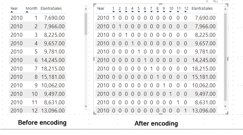
As you can see we have one new binary variable for each month, I didn’t bother renaming each column but it’s always cleaner to do all the renaming once you’re happy with your final model.
Now let’s rerun the model with the encoding binary month variables
Note that I purposely omit the first month, since I wanted to reproduce the dummy encoding done by R which uses N-1 features to represent N (so 12 months -1). (Dummy encoding is mainly used instead of one hot encoding to avoid the dummy variable trap)
Now let’s run our new model and see if we get the same output as R:

As we can see our new model using the categorical variable month is now perfectly matching with the model built in R.
Model improvements
Adjusted R squared
As we saw in the output interpretation the coefficient of determination or also called R Squared is crucial information to interpret the significance of our model since it tells us how well our model fits the data.
However, the R-squared has some limitations, in fact, if we keep adding more variables to our model the R-squared will always increase or remain the same.
On the other hand, the adjusted R-Squared as its name implies will adjust the value of the r-squared and penalizes us for adding variables that do not improve the existing model.
The formula for the Adjusted R-Squared is as follows:

Here is the formula in DAX:
The current value of the adj R-Squared is quite lower than the R-Squared so we will try to remove a variable that is not significant to increase the adj R-Squared

Let’s remove the variable Queries
We will remove the variable “Queries” since we already know from the summary output of R that this variable is not significant.
We can now run our new model:
Linest Elentra Dummy Encoding Without Queries =
linest(elantra[ElantraSales],
elantra[Unemployment],
elantra[CPI_all],
elantra[CPI_energy],
elantra[Year],
elantra[2],
elantra[3],
elantra[4],
elantra[5],
elantra[6],
elantra[7],
elantra[8],
elantra[9],
elantra[10],
elantra[11],
elantra[12]
)
And here is the output of the new model.

We notice the following:
- Removing the Queries variable did not decrease the R-Squared at all which suggests that this variable was in fact not significant
- The adjusted R-Squared has slightly increased so our model should perform better on real data
- The F-statistic has also increased which indicates that our model is more statistically significant
Identify significant variables
If we were only using the output of the Linest function in Power BI we would need to remove and add back each variable one by one to see which one penalizes our model the most.
However, we can calculate the p-value of each variable to find out which variables are significant and not significant. To do so we can use the t-test which I have described in this post: Paired Test in Power BI using DAX
Since I have already covered the p-value and t-test in a previous post I’m not going to repeat myself but in a short the small the p-value is the more statistically significant the variable will be for our model so any variables not significant can usually be removed from the model.
Here is the DAX code to calculate the p-value of the variable Queries of the multiple linear regression model that I called ‘Linest Elentra Dummy Encoding’.
And here is the output, I’m only showing 3 variables to show that the Power BI result matches with the R result.

Predict with the new model
Let’s now compare the prediction of our first model vs the final adjusted model we will predict the sales and compare the predicted sales vs the actual sales. Our model has been trained on 4 years of data from 2010 to 2013. We will see how our model fits the data on which it has been trained and also on new unknown data on which it has not been trained (first 2 months of 2014).
I have loaded a new table in my Power BI which contains the 2 new rows of the year 2014.
Predict the Sales with the multiple linear regression model:
We create a new column called “Predicted Sales” which is based on the first multiple linear regression model:
Then we create a second column to predict the sales based on the final adjusted model:
And here is the result of the two multiple linear regression model predicted sales vs actual sales:

As we can see the adjusted model performed much better in predicting the sales than the first model, however, for the last 2 months our model is not performing so well which is quite common in machine learning. The model tends to always perform better on trained datasets (2001 to 2013) than on test datasets (2014 data).
This is also why it is important to retrain the model frequently to avoid model drift (the model becomes less accurate over time).
Current limitations
There are currently a few limitations to implementing Multiple Linear Regression in Power BI but as we saw we can always work them around:
- Only numerical variables can be used but we can reencode the categorical variables into binary variables, this is tedious but it works
- The p-value is missing from the output table even if the F-stat can be used to reject the null hypothesis, the p-value is usually more commonly used
- The significance of each independent variable is missing but we can compute them manually
- The adjusted R-Squared is missing but we can easily compute it as well
Conclusion
This post was a shallow introduction to Multiple Linear Regression, it is, of course, impossible to cover all the aspects of Multiple Linear Regression in just a post as there are entire books written on this subject.
However, I wanted to show that since the new Linest function came out we can now easily implement it using Power BI and DAX only. It misses some output information that makes the model easier to interpret and fine-tune compared to R or other statistical tools but the missing metrics can easily be manually computed and added to the model. Overall I’m quite impressed with this new function and I wonder what will be the next function to come…
If you have read some of my posts about Statistics Using DAX only such as AB testing in Power BI, you know that I’m a big fan of applying statistical analysis using DAX only so this post again demonstrates that even if Power BI is not a statistical tool it has great statistical analysis capabilities and it just keeps getting better.
16 thoughts on “Multiple Linear Regression in Power BI”
Ben’s,
Is there any way you can attach the elantra.csv
So, I can follow your code please?
Thanks,
Oded Dror
hi Oded,
Yes sure here is the link to get the file:
https://github.com/f-benoit/PowerBI_Dataset/blob/main/elantra.csv
You need to filter out the two rows of 2014 until the prediction part of the blog.
I will add the pbix file soon, it’s just the file is too messy at the moment so I need to do some cleansing first
I did the month name and I stock in Linest Elentra Dummy Encoding?
Do I need to create 12 columns?
hi Oded,
yes if you want to use the month inside your model the months need to be pivoted and reencoded as explained in the blog.
To achieve the reencoding I used power query
– first step add index column
– then add custom column with all values=1
– then pivot the month column on the Dummy column
– then replace all null values by zero
#”Added Custom” = Table.AddColumn(#”Changed Type”, “Dummy”, each 1),
#”Added Index” = Table.AddIndexColumn(#”Added Custom”, “Index”, 0, 1, Int64.Type),
#”Pivoted Column” = Table.Pivot(#”Added Index”, List.Distinct(#”Added Index”[month]), “month”, “Dummy”, List.Sum),
#”Replaced Value” = Table.ReplaceValue(#”Pivoted Column”,null,0,Replacer.ReplaceValue,{“1”, “2”, “3”, “4”, “5”, “6”, “7”, “8”, “9”, “10”, “11”, “12”})
This will generate 12 new columns called 1,2,3,4,5… each corresponding to the month
I’m getting error The column ‘month’ of the table wasn’t found.
Details:
month
Here is my PQ steps:
let
Source = Csv.Document(File.Contents(“C:\PowerBI\Videos\BEN’s Blog\PowerBI-main\Elantra.csv”),[Delimiter=”,”, Columns=8, Encoding=1252, QuoteStyle=QuoteStyle.None]),
#”Promoted Headers” = Table.PromoteHeaders(Source, [PromoteAllScalars=true]),
#”Changed Type” = Table.TransformColumnTypes(#”Promoted Headers”,{{“Month”, Int64.Type}, {“Year”, Int64.Type}, {“ElantraSales”, Int64.Type}, {“Unemployment”, type number}, {“Queries”, Int64.Type}, {“CPI_energy”, type number}, {“CPI_all”, type number}, {“”, type text}}),
#”Added Custom” = Table.AddColumn(#”Changed Type”, “Dummy”, each 1),
#”Added Index” = Table.AddIndexColumn(#”Added Custom”, “Index”, 0, 1, Int64.Type),
#”Pivoted Column” = Table.Pivot(#”Added Index”, List.Distinct(#”Added Index”[month]), “month”, “Dummy”, List.Sum),
#”Replaced Value” = Table.ReplaceValue(#”Pivoted Column”,null,0,Replacer.ReplaceValue,{“1”, “2”, “3”, “4”, “5”, “6”, “7”, “8”, “9”, “10”, “11”, “12”})
in
#”Replaced Value”
Hi Oded
Power query is capital sensitive I can see that first month is “Month” while in th other step it is “month”
hi Oded,
you can refer to this post where I break down each step to perform the dummy encoding:
https://datakuity.com/2023/03/15/one-hot-encoding-in-power-bi/
Another thought, columns are naturally static
and we are looking at dynamic slicers. just wondering is that approach ok?
Would you be able to go through an example with LINESTX using virtual tables?
Hi,
Firstly, you did an excellent job of explaining the new project to the team, your presentation was well explained and easy to follow. Thank you so much you helped me a lot.
But could you please share the file in powerBI?
Please help me. Thank you
Hi Hadirah,
Thanks for the comment here is the PBIX file: https://github.com/f-benoit/PowerBI/raw/main/Multiple%20Linear%20Regression/Multiple%20Linear%20Regression%20with%20Linest.pbix
Hi,
Firstly, you did an excellent job of explaining the multiple linear regression, your writing was well explained and easy to follow. Thank you so much you helped me a lot.
But could you please share the file in powerBI?
Please help me. Thank you
It is a really great job!.
One more request here is that ‘Can you add country as a column ?’ And I would like to see comparison by each countries and makes visualization of each trend-line in power bi.
I want to implement a linear regression for grouping data.
Thank you so much in advance
Wow, that’s a super cool post, Ben! Especially about the Linest function.
Thanks for sharing your knowledge,
Franco
Thanks for the blog post. It helped me very much with my task at hand. Do you by any chance know of a DAX way to do a logarithmic regression instead of a linear?
best Regards