In this post, I will share how to perform a bootstrap analysis with Power BI.
I will briefly introduce what is bootstrapping and when to use it.
For more details I will add some reference links at the end of this post.

What is Bootstrapping?

The bootstrap method is a resampling technique used to estimate statistics on a population by creating many simulated samples. It can be used to estimate summary statistics such as mean, standard errors, construct confidence intervals and thus perform hypothesis testing

How the Bootstrap method works?

As seen above the bootstrap method is used to estimate a quantity of a population.
This is achieved by repeatedly taking small samples from a large sample, calculating the statistic and then taking the average of the calculated statistics.

• Choose the number of bootstrap samples to take
• Choose the sample size “n”
• For each sample
  • Draw a sample with replacement with the chosen size
  • Compute the statistic of the sample
• Calculate the mean of all the calculated sample statistics.

Why to use Bootstrap analysis with Power BI?

Both bootstrapping and traditional methods use samples to draw inferences about populations.

However, as the opposite of most traditional statistical methods bootstrapping method does not require assuming any parametric form for the population distribution.
So one of the greatest advantage of bootstrap is its simplicity and its straightforward way to derive estimates of mean or standard error whatever the distribution of the data might be.

So why using Power BI?

• First you may not have R or Python developer within your team
• Since Bootstrap works great with small samples size it’s likely that the Power Bi engine will easily handle the computation.
• For advanced statistical analysis, Power BI may not be the go-to tool; however to perform a bootstrap analysis we don’t need any specific statistical tool, and Power BI can do the job.
• Building everything with Power BI allows us to keep the interaction across each visual.
• Easier to maintain.

How to perform a Bootstrap analysis with Power BI?

The data

The dataset can be found here: https://www.kaggle.com/arpitdw/cokie-cats
The project can also be found on Datacamp using Python.

Cookie Cats is a mobile puzzle game, it’s a “connect three”-style puzzle game where the player must connect tiles of the same colour to clear the board and win the level.

As players progress through the game they will encounter gates that force them to wait sometime before they can progress or make an in-app purchase.

In this post, using Bootstrap analysis with Power BI we will analyze the result of an A/B test where the first gate in Cookie Cats was moved from level 30 to level 40. In particular, we will analyze the impact on player retention.

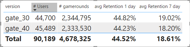
First 10 rows:

Retention_1: True if the player came back and play 1 day after installing
Retention_7: True if the player came back and play 7 day after installing
Version: Whether the player was put in the control group (Gate30) or the tested group (Gate40)
Sum_Gamerounds: The number of game rounds played by the player

The distribution of game rounds

It looks like there is around the same number of players in each group.
The retention in the group Gate30 is slightly better than the group in the Gate40.

avg Retention 1 day = AVERAGE(cookie_cats[Retention_1Day])

Overall 1 day retention

As we can see from the line chart above:

• Some players installed the game but never played it
• Some players played only one round and then never played it again
• Some players played a couple of games in their first week
• Some players really loved it and played many rounds

A common metric in the video gaming industry for how engaging a game is 1-day retention: The percentage of players that comes back and plays the game one day after they have installed it. The higher 1-day retention is, the easier it is to retain players and build a large player base.

# Users = DISTINCTCOUNT(cookie_cats[userid])

Generate Bootstrap Samples

In order to generate the bootstrap samples we need to define:

• Number of samples: _nb_samples=500
• Sample Size: _frac=10/_nb_samples*COUNTROWS(cookie_cats)

We create a calculated table to generate the new dataset based on 500 samples drawn from the original sample.

bootstrap = 
var _nb_samples=500
var _min_idx = min(cookie_cats[Index])
var _max_idx = max(cookie_cats[Index])
var _frac = 10/_nb_samples*COUNTROWS(cookie_cats)


// Generate an array of number of samples
VAR _array_samples= SELECTCOLUMNS ( GENERATESERIES ( 1,_nb_samples), "_sample", [Value] )
// Generate an array of sample size
VAR _array_frac= SELECTCOLUMNS ( GENERATESERIES ( 1,_frac), "_frac", [Value] )

//new table number of rows=_nb_samples*_frac 
var _cross_samples_frac =CROSSJOIN(_array_samples,_array_frac) 
    
//add random idx
VAR _randIdx_Table = ADDCOLUMNS(_cross_samples_frac, "_idx", int(RANDBETWEEN(_min_idx,_max_idx)))

//add src table
VAR _src_table =
    SELECTCOLUMNS (
        cookie_cats,
        "_idx", int(cookie_cats[Index]),
        "version", cookie_cats[version],
        "retention_1day",cookie_cats[Retention_1Day],
        "retention_7days",cookie_cats[Retention_7Days]
    )

//join two tables
VAR _src_join_randIdx = NATURALINNERJOIN(_randIdx_Table,_src_table)

var _groupby = GROUPBY(  
                     _src_join_randIdx
                    ,[_sample]
                    ,[version]
                    ,"AVG_Retention_1Day", AVERAGEX(CURRENTGROUP() ,[retention_1day])  
                    ,"AVG_Retention_7Day", AVERAGEX(CURRENTGROUP() ,[retention_7days])  
                    )  
return
_groupby

Ok let’s break down the code above.

1. First we set the variables
   1. Samples size, number of sample,
   2. _min_idx and _max_idx will be used to generate random indexes between min and max
2. Then we create two arrays
   1. One array of the number of samples
   2. One array of the sample size chosen
3. We cross join the two arrays to get a table with number fo rows= _nb_samples*_frac
4. We add a new column to the table _randIdx_Table which generate a random int for each row (random int between _min_idx and _max_idx)
5. We create a variable “_src_table” that holds the source table with only the selected columns
6. We join the two tables _randIdx_Table and _src_table
7. We create a new variable “_groupby” which aggregate the retention value by Sample and version
8. We return the calculated table

Sample Avergae Distribution

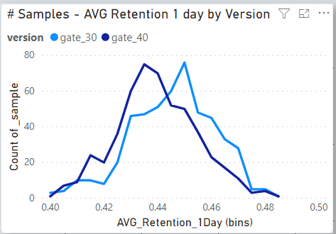
The above chart shows the two distributions of the bootstrap samples for 1 Day of Retention.
These distributions represents the uncertainty over what the underlying 1-day retention could be.
By looking at the chart we can see that there seems to be some evidence that Gate 30 performs better than Gate 40.
Now let’s examine the difference in 1-day retention.

Distribution of the 1 Day Retention Difference

From this chart, we can see that the distribution seems to be slightly in favour of a gate at level 30. But what is the probability that the difference is above 0%? Let’s examine in details the difference in % between Gate 30 and Gate 40.

AVG_1Day_Diff = 
      var avg30 = CALCULATE(AVERAGE(bootstrap5[AVG_Retention_1Day]), bootstrap5[version]= "Gate_30",ALLEXCEPT (bootstrap5,bootstrap5[_sample] ))
      var avg40 = CALCULATE(AVERAGE(bootstrap5[AVG_Retention_1Day]), bootstrap5[version]= "Gate_40",ALLEXCEPT (bootstrap5,bootstrap5[_sample] ))
      return 
      Divide(avg30-avg40,avg40)*100 

So overall a gate at level 30 is 1.49% higher than a gate at level 40.

Probability of a difference

So we saw that a gate at level 30 seems to have a better 1-day retention of around 1.5%.
Now we want to find out how likely that the difference will be above 0%? 

So by setting the gate at level 30 has about 60% more chance to retain players than setting the gate at level 40.

Prob_1Day_Diff = 
var _prod=calculate(COUNTROWS(bootstrap),bootstrap[AVG_1Day_Diff]>0)
var _len =COUNTROWS(bootstrap)
return
divide(_prod,_len)

To Recap

The bootstrap result tells us that there is a bit of evidence that 1-day retention is higher when the gate is at level 30 than when it is at level 40.

The conclusion could be:
If we want to keep 1-day retention high we should not move the gate from level 30 to level 40.
There are, of course, other metrics that could be analysed such as number of in-game purchases, number of game round…

The aim of this post was not to go into details about the use of the bootstrap method but rather to show how we can easily implement a bootstrap analysis with Power BI.

Further Readings

• AB Testing WIth Power BI: https://datakuity.com/2020/09/29/ab-testing-with-power-bi/
• Bootstrapping: Wikipedia
• A Gentle Introduction to the Bootstrap Method Using Python
• Central Limit Theorem with R: https://datakuity.com/2018/01/07/central-limit-theorem-example-using-r/