Central Limit Theorem -example using R
The Central Limit Theorem is probably the most important theorem in statistics. In this post I’ll try to demystify the CLT with clear examples using R.
The central limit theorem (CLT) states that given a sufficiently large sample size from a population with a finite level of variance, the mean of all samples from the same population will be approximately equal to the mean of the original population.
Furthermore, the CLT states that as you increase the number of samples and the sample size the better the distribution of all of the sample means will approximate a normal distribution (a “bell curve“) even if the original variables themselves are not normally distributed.
Let’s break down this with some examples using R:
Table of Contents
Central Limit Theorem – example using R
Original Population with a left-skewed distribution
Let’s generate our left-skewed distribution in R.
By using the rbeta function below I generated 10,000 random variables between 0 and 1 and I deliberately changed the shape parameter to have a distribution with a negative skewness.
myRandomVariables<-rbeta(10000,5,2)*10

The mean (µ) of the total population is 7.13 and the standard deviation (σ) is 1.61.
We can see that the distribution has a tail longer on the left with some data that go up to 4 standard deviations away from the mean whereas the data on the right don’t go beyond 2σ away from the mean.
As we can see on the plot above the standard deviation (σ) allow us to see how far away from the mean each data are.
A small σ means that the values in a statistical data set are close to the mean of the data set, on average, and a large σ means that the values in the data set are farther away from the mean, on average.
AS the σ is 1.61 it means that all the data between 5.52 (7.13-1.61) and 8.74 (7.13+1.61) are close to the mean (less than 1 σ).
However, the data less than 2.30 (7.13-3*1.61) are much more far from the mean at least 3σ.
To better illustrate let’s see the same plot with the data scaled such as the mean is equal to 0 and the standard deviation is equal to 1.
The formula to get the data normalised is (x-µ) / σ
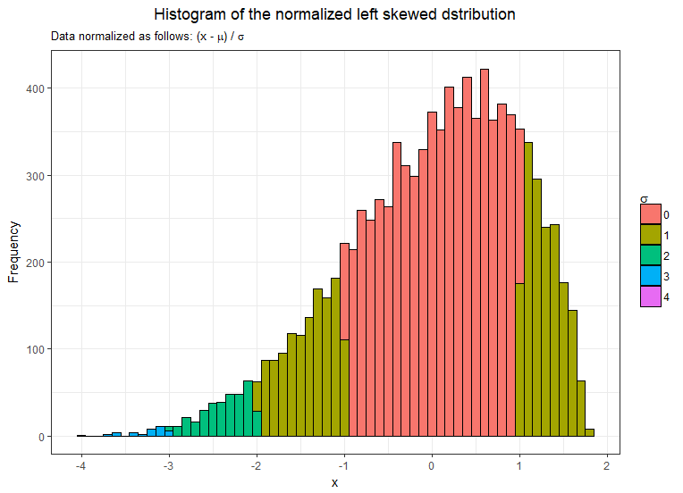
The distribution still has exactly the same shape but it just makes it easier to observe how the data are close or far from the mean.
Using the Central Limit Theorem to Construct the Sampling Distribution
So how can we use the CLT to construct the sampling distribution? We’ll use what we know about the population and our proposed sample size to sketch the theoretical
sampling distribution.
The CLT states that:
- The shape of the sampling distribution: As long as our sample size is sufficiently large (>=30 is the most common but some textbook use 20 or 50) we should assume the distribution of the sample means to be approximately normal disregarding the shape of the original distribution.
- The mean of the distribution (x̅): The mean of the sampling distribution should be equal to the mean of the original distribution.
- The standard error of the distribution (σx): The standard deviation of the sample means can be estimated by dividing the standard deviation of the original population by the square root of the sample size. σx = σ/√n
Let’s prove it then!
I will first draw 100 mean samples from the original population with the minimum size recommended by the CLT 30.
Here is the code to generate the sample means:

So according to the CLT theorem, the three following statements should be true:
- The mean of our sample means distribution should be around 7.13
- The shape of the sample distribution should be approximately normal
- Standard error (σx = σ/√n) should be equal to 0.29 (1.61/√30)
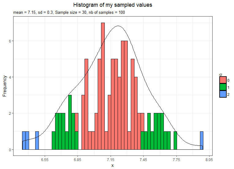
- The mean is 7.15 hence nearly 7.13
- The shape is approximately normal still a little bit left-skewed
- The standard error is 0.3 hence nearly 0.29
The CLT also states that as you increase the number of samples the better the distribution of all of the sample means will approximate a normal distribution.
Let’s draw more samples.
Now I take 1,000 samples means and plot them.

- The mean is still 7.15 and not exactly 7.13
- The shape is approximately normal but still a little bit left-skewed
- The standard error is equal to 0.29 as estimated by the CLT theorem
Let’s take even more sample means.
This time I take 10,000 samples means and plot them.
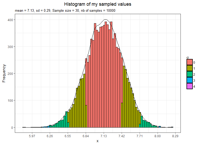
- The mean is now exactly 7.13
- The distribution shape is definitely normal
- The standard error is equal to 0.29 as estimated by the CLT theorem
Just for the fun let’s do another example and this time with a different sample size to see if we get the standard error right.
So using the CLT theorem the σx should be 0.11 (1.61/√200)
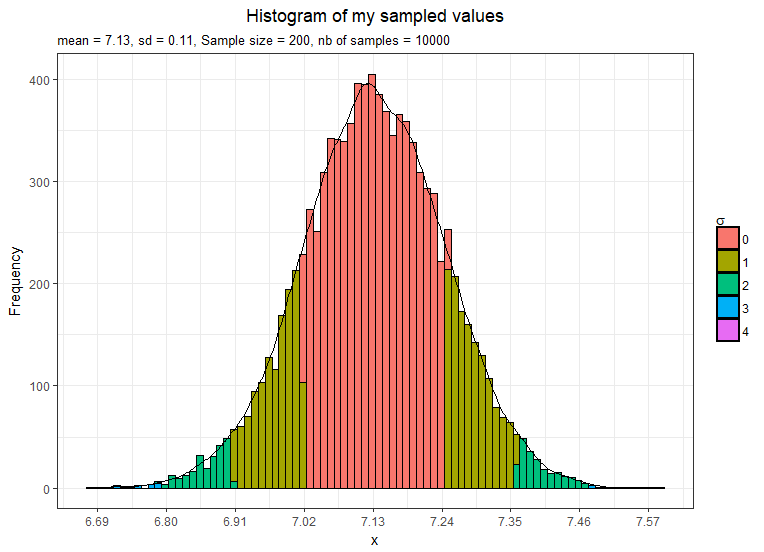
We have increased each sample size to 200 instead of 30 in the previous examples hence the variance in the sample means distribution has decreased and we now have a standard error smaller.
This confirms that as we increase the sample size the distribution becomes more normal and also the curve becomes taller and narrower.
Summary
The CLT confirms the intuitive notion that as we take more samples or as we increase the sample size, the distribution of the sample means will begin to approximate a normal distribution even if the original variables themselves are not normally distributed, with the mean equal to the mean of the original population (x̅=µ) and the standard deviation of the sampling distribution equal to the standard deviation of original the population divided by the square root of the sample size (σx = σ/√n).
In the next post I’ll talk more in-depth about the CLT and we’ll see how and where we can use the CLT.
15 thoughts on “Central Limit Theorem -example using R”
Sorry, can I get the code for R? Thanks
Hi Alfira,
Sure send me your email via the contact form and I’ll send the r script to you
can i get the r code too?
faziraputeri99@gmail,com
Can I get the R code too?
nguyenquocduongqnu1999@gmail.com
Hi –
Fantastic explanation using R. Would it be possible to receive the R code that you used?
Hi Anthony,
Yes sure, please send me your email so I can send it to you.
Hello Ben,
Would it be possible to request your R codes you used?
Thank you
Hi Ben, thanks, can i get the R code, please? thanks anam.vielma@gmail.com
Hi Ana,
I just sent you the code
Hey Ben, would it be possible to get the R-Code you used here?
Thanks.
Hey Vita,
sure you can get part of the code here: https://raw.githubusercontent.com/f-benoit/Statistics/main/CLT.r
you can ply the parameters to get different results:
n<-500 sampSize<-200
hey! can i get the R code?
Hi you can get the code here: https://raw.githubusercontent.com/f-benoit/Statistics/main/CLT.r
Hi can I also get the R code please
thanks